Today we are going to explain how to set conditional formatting based on another cell in Google Sheets. Conditional formatting is a function in Google Sheets that displays a cell in a specific way when certain conditions are met. The behavior of the cell’s format may be altered, including highlighting, bolding, or italicizing.
If you are wondering how to use the Excel COUNTIF formula, don’t forget to visit our guide. Now let’s review conditional formatting based on another cell in Google Sheets.
How conditional formatting works in Google Sheets?
Let’s use this spreadsheet as an example to learn how to use conditional formatting.
 It’s a spreadsheet that displays yearly website traffic from Q4 2020 to Q4 2021, including page views and year-over-year percentage change.
Here’s what we’re aiming for: When the percentage change is positive YoY, the cell goes green. When it’s negative, the cell becomes red. This makes it simple to get a brief performance assessment before delving further into the data.
Set the conditional formatting by following these steps:
Step 1: Choose the cell you wish to format, then click on “Format” from the navigation bar, followed by “Conditional Formatting.”
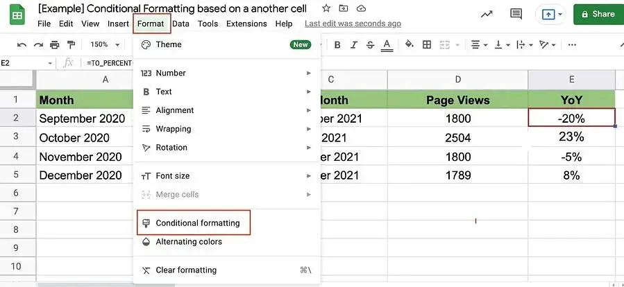 Step 2: Stay in the “Single color” tab, and now check that the cell under “Apply to range” is the cell you wish to format.
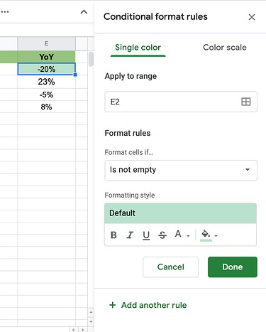 Step 3: Assign format rules.
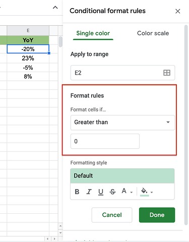 Step 4: It may immediately select a common condition format. In this situation, choose your rules from the dropdown menu under “Format cells if…” These are your options:
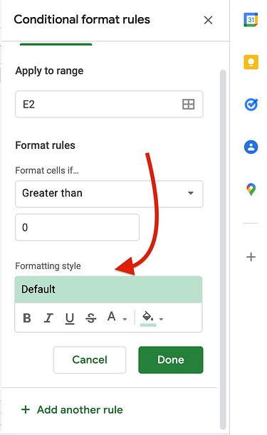 Step 5: Choose your preferred style, then select “Done.”
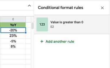 Step 6: Confirm the rule was applied under “Conditional Formatting Rules.”
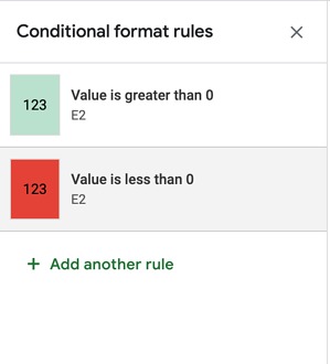 Step 7: Add another rule if you need it.
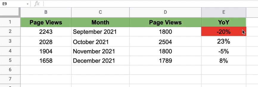 Step 8: To format a cell, choose the desired style from the drop-down menu, then click to select it. Then drag the cursor over other cells to apply your formatting.
These are the basics. Now let’s learn how to use conditional formatting based on another cell.
Conditional formatting based on another cell value
Step 1: Choose the cell you wish to format
 Step 2: Click on “Format” from the navigation bar, followed by “Conditional Formatting.”

Step 3: Under “Format Rules,” choose “Custom formula is.”
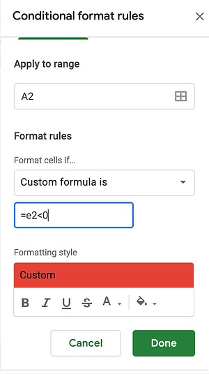 Step 4: Type in your formula, then select “Done.”
Conditional formatting based on another cell range
To format based on another cell range, you follow many of the same steps you would for a cell value. What changes is the formula you write.
 Step 1: Choose the cell you wish to format

Step 2: Click on “Format” from the navigation bar, followed by “Conditional Formatting.”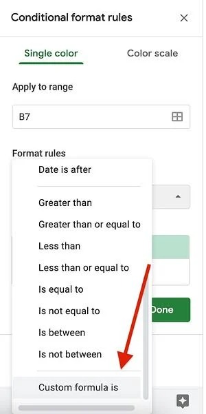
Step 3: Under “Format Rules,” choose “Custom formula is.”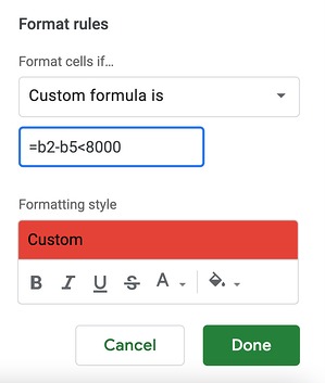
Step 4: Type in your formula using the following format: =value range < [value], select your formatting style
Step 5: Select “Done.”
Conditional formatting based on another cell color
There is no way to use condition formatting in Google Sheets based on the color of another cell, at present. You can only utilize it for:
- Values
- Text
- Dates
- Emptiness
To reach your objective, you’d need to utilize the cell’s condition to format the other.
Let’s use an example.
 Step 1: Suppose you want to color cell A2 (September 2020) red and match the color of cell E2 (-20). There is no formula that allows you to create a condition based on color. However, you can make a custom formula based on E2’s values.
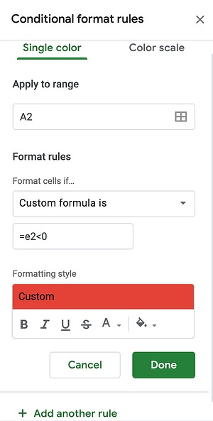 Step 2: If cell E2’s values are less than 0, the color of cell A2 changes. The formula is as follows: = [The other cell] < [value]. In this case, the formula would be e2e0n, as it indicates that column A should become red if E2’s value is less than 0.
Google Sheets may appear complex when you have so many features to experiment with. You can quickly format your cells using these simple instructions if you’re intimidated by Google Sheets.
This way you’ve learned basic elements of conditional formatting based on another cell in Google Sheets. If you want to learn how to merge cells in Google Sheets, we are here to help.


