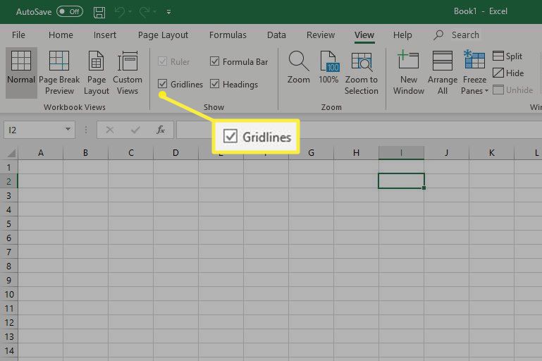
If you don’t know how to print gridlines in a worksheet in Excel, we are going to help you out in this step by step guide. When you work in Microsoft Excel, there are gridlines that separate rows and columns in cells. These light gray lines keep the data organized and easy to read. When you go to print your Excel spreadsheet, it will print the document without gridlines by default unless you change the settings.
How to print gridlines in a worksheet in Excel?
 If you want to see those gridlines on the page you are going to print, follow these steps:
- Launch Microsoft Excel and open a worksheet.
- Select the “File” menu and click on “Page Setup…” and within this dialog box, you can choose the settings that apply to the entire Excel worksheet.
- Click on the “Sheet” tab at the top of the “Page Setup” dialog box to display the values.
- Find the “Print” section of the “Sheet” tab in the “Page Setup” dialog box, which is located in the center of the dialog box.

- Use your mouse to click the checkbox in front of the “Gridlines” option to add a checkmark to the box. This will ensure that the gridlines will print when printing the current document.
- Click the “OK” button.
- Print the worksheet. Enter the “File” menu, click on “Print” and then you will notice that the gridlines will be printed as well.


