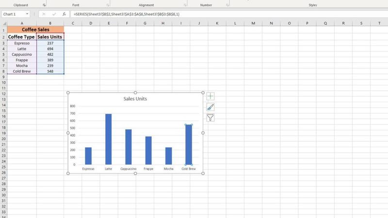
If you want to know how to change the series name in Excel, please read below.
Microsoft Excel is one of those tools that many of us use daily. Or at least once a week. The thing is that we tend to waste time performing actions manually when we could carry them out using certain shortcuts. On this particular occasion, we intend to show you how to rename a data series in Excel. This is a really useful trick, so pay attention to it.
As we said before, the following tutorial will give you a hand especially in those cases in which you want to change or edit the name of a data series in an Excel chart. The idea is to modify those contents without changing the elements that appear in the rows or columns. And what are data series? They refer to the data that appear at the bottom of the chart or table. They can be the names of rows or columns.
Best of all, it is a fairly straightforward process. Creating a bar chart or a plain chart in Excel is not too complicated. When we do so, we get information about the selected cells. If you’ve gotten that far, let’s see how to modify that data.
How to change the series name in Excel?
To edit or rename a data series in a Microsoft Excel chart or graph without editing the name of the original row or column, you have to follow these steps that we are going to show you:
- Open Excel on your computer.
- Open the Excel spreadsheet where the chart is located.
- Select the chart.
- Right-click on it and choose the option Select data.
- Select the data series in the Legend entries box.
- Click on Edit.
- Enter the new name in the Series name box.
- Add the values of the series if you consider it necessary.
- Click on OK.
At this point, you have to open the Excel spreadsheet where you can find the desired chart. Then, select the chart in the spreadsheet and right-click on it. In the context menu, an option called Select data will appear. You have to click on it.
After that, choose the name of the data series you want to change in the Legend entries box that appears on the left side of the screen. Later, you have to click on the Edit button.
Now, delete all the contents of the Series name box and enter the new names you want to display in the chart. After that, enter the Series values if you want to customize them further.

Once you have finished all the previous steps, click the OK button twice to save the changes. After saving, the spreadsheet chart will appear with the name of the new data series. As you can see, this is a fairly simple procedure, which does not bring any great difficulties.
If you have found this article useful, you will probably like to know more tutorials related to this application of Microsoft’s office suite. For example, how to add a title line in an Excel spreadsheet.


